This post is part of a series on category theory. See Overview of Blog Posts for a list of all posts. All categories in this post are assumed to be locally small (the morphisms between two objects form a set), unless stated otherwise.
Introduction
Last time, we studied universal properties and representable functors. A particular class of universal properties and representable functors is given by (co)limits. This class generalizes many known and frequently appearing constructions and is of great importance both for the study of categories themselves and for applications of category theory. Using the notion of limits, we will be able to state and prove a useful criterion for when a functor is representable in a future post. For motivation, we will start be studying particular examples of limits and colimits in familiar categories before giving the general definition in the future. As we shall see in future posts, all general limits and colimits can be constructed from these examples.
Terminal and Initial Objects
We have already defined initial objects in definition C5.12, but for completeness’s sake, we shall repeat the definition here.
Definition C6.1 Let  be a category. Then an object
  is called terminal if for any object
  , there is a unique morphism
  .
.
Definition C6.2 Let be a category. Then an object  is called initial if for any object , there is a unique morphism
  .
.
Remark From the definitions, it is clear that an initial object is just a terminal object in the opposite category and vice versa.
Remark By lemma C5.13, intial objects (and hence terminal objects, see above) are unique up to unique isomorphisms.
Example C6.3 In the category of sets, the empty set  is the unique initial object. Indeed, for any set
  , there is a unique map
  , namely the empty map. Every one-point set
  is a terminal object, as for any set , there is a unique map
  that sends everything to
  . Similarly, in the category
  of topological spaces, the empty space is an initial object and the one-point space is a terminal object. In the category of small categories
  , the empty category is an initial object and the category with one object and one morphism (the identity of the one object), i.e. a one-object discrete category, is the terminal object.
Example C6.4 In the category of groups, abelian groups, or modules over a ring  , the trivial group (or zero module module) is both an initial and a terminal object.
Example C6.5 In the category of rings, the zero ring  is a terminal object and the ring of integers
  is an initial object. More generally, let be a commutative ring and consider the category of -algebras. Then is an initial object and the zero ring is a terminal object. This generalizes the last example, as rings are equivalently -algebras.
Example C6.6 Let  be a preordered set, considered as a category (cf. example C1.5). Then an initial object is an element
  , such that
  for all
  , i.e. a least element. Dually, a terminal object is a greatest element.
Example C6.7 The category of fields does not have an initial object or a terminal object. The reason is that if two fields have different characteristic, there is no field homomorphism between them. If we fix the characteristic to be or a prime number  , then the category of fields of that characteristic has the prime field of that characteristic, i.e.
  or
or  as an initial object, but it still has no terminal object, as all field homomorphisms are injective and there are fields of arbitrarily large cardinality.
Remark In the terminology of universal properties and representable functors, an initial object in represents the constant functor  that sends every object to the terminal object in
  , namely a one-point set. The identity of the initial object is a universal element for this constant functor. Dually, a terminal object represents the constant functor that sends everything to a one-point set, considered as a contravariant functor, i.e. a functor
  . The identity of the terminal object is a universal element.
Products and Coproducts
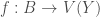
Definition C6.8 Let be a set and let  be a collection of objects in a category . Then a product is given by the following data:
- An object in , denoted by

- A collection of morphisms, for any
 , a morphism
  , called structure morphisms or canonical projections.
With the following universal property:
- For any object
 in and a collection of morphisms
  , there exists a unique morphism
  such that
  for all
  .
.
The property can be visualized via a commutative diagram, here shown in the case of binary products: 
Remark C6.9 Let  be the empty set. Then a product
  is exactly a terminal object.
Example C6.10 Consider the category of sets . For a family of sets , one can construct the Cartesian product and let  be the projection onto the
  -th coordinate. This clearly satisfies the universal property for a product, as for any set and maps , the obvious definition
  yields the unique map
  such that
  for all . If we have the category of semigroups, of monoids, of groups, of abelian groups, of rings, of -modules or of -algebras etc. with their respective homomorphisms as morphisms, then equipping the cartesian product with coordinate-wise operations yields the product in that category. (Note that as the operation in the product is defined coordinate-wise, the projections are homomorphisms of the respective type of algebraic structure.)
In the category of topological spaces , one takes the Cartesian product and equips it with the product topology to obtain the categorical product.
Example C6.11 Let be a preordered set. Then the product of a family of objects, if if it exists, is the infimum. The universal property of the product turns into the universal property of the infimum:  . For example, if
  is an integral domain and we define
  if and only if
  divides
  , then the product will be the greatest common divisor of a family of objects, if it exists.
Example C6.12 Consider the category of small categories . Then for a family of categories  , there’s the product category
  together with projection functors
  for all . The objects are given by
  and the morphisms are given by
  with composition defined component-wise. We have already seen the special case for binary products in definition C3.7.
Remark Let be a category and let be a family of objects indexed by a set . Then if the product  , exists, we have a bijection for any object ,
 , given by
  , where the
  are the structure morphisms of the product. One checks that this is natural in . This means that the functor
  is represented by and that the family of structure morphisms
  is a universal element. Thus we have shown that the “universal property” of the product is indeed a universal property in the formal sense defined in the last entry.
Conversely, given a representation of the functor  , the representing object is a product of the
  and the universal element is the family of structure morphisms.
Being representing object of a functor, a product is uniquely determined up to unique isomorphism in the following sense: If and  are products for the family with structure morphisms
  and
and  , then there exists a unique isomorphism
  such that
  for all .
As with any notion defined for a category, we can dualize the concept of a product.
Definition C6.13 Let be a category, let be a set and let be a family of objects in . Then a coproduct of is a product of in  . The coproduct is denoted by
  , the structure morphisms
  are also called canonical inclusions.
Exercise Write out the universal property of coproducts as in definition C6.8.
Remark Dualizing a previous remark, a coproduct over an empty set is equivalently an inital object.
Example C6.14 Consider the category of sets . The coproduct of a familiy of sets is given by the disjoint union  and the structure morphisms are given by the inclusions
  . The universal property of the coproduct says that having a map defined on a disjoint union
  is equivalent to having a map
  for each . The correspondence is given by composing with inclusion, i.e. restricting to each component of the disjoint union.
In the category of topological spaces, we can also take the disjoint union with the finest topology that makes all inclusions continuous.
Similarly, in the category of small categories, one can take the disjoint union of objects and the disjoint union of morphisms to get coproducts. (E.g. any discrete category is a disjoint union of copies of the terminal category. The category of fields is a disjoint union of the categories of fields of a fixed characteristic  , where varies over all primes and .)
Example C6.15 Let be a ring and consider the category of left -modules  . For a family of left -modules
  , the direct sum
  (i.e. the submodule of the product consisting of all tuples in which all but finitely many entries are ) is the coproduct with the structure morphisms
  given by the inclusion in the j-th coordinate. Note that for a finite family, product and coproduct agree, although the structure morphisms are different.
Example C6.16 Consider the categeory of groups  . Here the coproduct is given by the so-called free product. For simplicity, let us define the free product in terms of presentations (as it satisfies a universal property, it is unique up to unique isomorphism and hence doesn’t depend on the presentation.) If
  is a family of groups with presentations
  , then the free product has a presentation
  and the structure morphisms are induced by the inclusion of generators
  . (cf. example C5.5 for the universal property of presentations.)
Example C6.17 Dualizing example C6.11, if we consider a preordered set as a category, then the coproduct of a family of objects is given by the supremum, if it exists. For the divisibility relation in an integral domain, this is the least common multiple.
Remark Just like with products, coproducts can be understood in terms of representable functors (they are just products in the opposite category, after all). Explicitly, for a family of objects  in a category , we can form the product of Hom-functors
  . A representation of this functor is equivalently a coproduct, with the universal element being the family of structure morphisms. (cf. the corresponding remark for products.)
Equalizers and Coequalizers
Definition C6.17 Let  be a category, let
  be objects and let
  be a family of morphisms. Then an equalizer
  consists of the following data:
- An object
 in
in
- A morphism
 , called structure morphism or -by abuse of terminology- also the equalizer of the
  , which satisfies
  .
.
Such that the following universal property holds:
- For any object
 and every morphism
  such that
  , there is a unique morphism
  such that
The universal property can be visualized via a commutative diagram, here shown in the case of binary equalizers:

Remark Equalizers are terminal objects in a suitable chosen category: in the situation of definition C6.17, define the following category  :
:
- Objects are pairs
 where is an object in and
  is a morphism such that
  .
.
- Morphisms
 are morphisms
  in such that
- Composition is inherited from
Then one may restate the definition of an equalizer by saying that an object  is a terminal object if and only if
  is an equalizer with structure morphism
  . This implies that an equalizer is unique up to unique isomorphism in the following sense: If and
  are both equalizers of the same family of morphisms
  , then there exists a unique isomorphism
  such that
  .
.
Example C6.18 Consider the category of sets . Then an equalizer of a family of maps  can be realized as the largest subset of on which they agree: If we let be the subset of consisting of all such that
  and take to be the subset inclusion, then any map such that
  has its image contained in . Hence it factorizes uniquely through the subset inclusion , showing that satisfies the universal property. If all sets involved are semigroups, monoids, groups, rings or -modules etc. and the maps are homomorphisms of the respective type, then will be a subsemigroup, submonoid, subgroup, subring or submodule, respectively and by the same argument, satisfies the universal property of the equalizer.
Suppose a group  acts on a set , then we can consider the action as a collection of maps
  . In this case, one checks that the set is given by the set of invariants
  .
.
One can think the equalizer as measuring “how equal” a collection of morphisms are.
Definition C6.19 A coequalizer in a category is an equalizer in the opposite category  .
.
Exercise Write out the universal property for coequalizers.
Example C6.20 Consider the category of sets , then a coequalizer of a family of morphisms ,  can be constructed as follows: Consider the equivalence relation
  on generated by
  for all
  and
and  . (Given a relation on a set, the intersection of all equivalence relations containing it is again an equivalence relation, called the equivalence relation generated by it.) Then the quotient map
  is a coequalizer. If a group acts on a set , then if we consider the coequalizer of the family of maps by which acts, this is the quotient space
  . If we use the quotient topology, the same construction works in the category of topological spaces.
Example C6.21 If we work in the category of -modules and we have a family of -linear maps  , then one can take the quotient of
  by the submodule generated by the set
  where
where  vary over and
  varies over
  . The quotient module with the quotient map is then a coequalizer in the category of -modules.
If one thinks of an equalizer as a universal solution to the problem of making maps equal from the left (i.e. by precomposing with a map), then dually a coequalizer is a universal solution to the problem of making maps equal from the right (i.e. by postcomposing with a map).
Pullbacks and Pushouts
Definition C6.22 Let be a category, let  be objects and let
  and
and  be morphisms. Then a pullback consists of the following data:
- An object

- Morphisms

Such that the following universal property holds:

- For every object
 and morphisms
  and
and  such that
  , there exists a unique morphism
  such that
  and
and 
The universal property can be visualized by the following commutative diagram: 
Exercise Generalize this definition to the case of a family of objects and a family of morphisms  .
.
One can think of pullbacks as a “mix” of products and equalizers. For products, we had multiple objects but no morphisms between them as a given datum, whereas for equalizers, we had multiple morphisms, but all with the same source and target. For pullbacks, we have different objects and morphisms from those objects to a common target. The following lemmata make the relation of pullbacks to equalizers and products precise.
Lemma C6.23 In the situation of definition C6.22, suppose that the product  exists and suppose that for the structure morphisms of the product
  and
and  , the equalizer
  exists with structure morphism
  . Then this equalizer is a pullback with structure morphisms
  and
and  .
.
Proof We verify the universal property. We have  from the definition of an equalizer. Let be an object and let and be morphisms such that
  . Then by the universal property of the product, there is a unique morphism
  such that
  and
and  . Then we get that
  , so that by the universal property of the equalizer, there is a unique map
  with the required property.
Lemma C6.24 Suppose that a category has a terminal object  . Then, if for two objects , the pullback
  (along the unique morphisms
  ), exists, it is a product of and .
Lemma C6.25 Suppose that in a category , the product  for an object exists. Let
  be two morphisms from another object and let
  be the unique morphism such that
  and
and  . Furthermore, let
  be the unique morphism such that
  and
and  . Then if the pullback
  exists, it is an equalizer
  with structure morphism defined via the projection
  .
.
Exercise Prove the preceeding two lemmata. (This is a nice exercise in getting used to working with universal properties.)
Exercise If a pullback exists, it is unique up to unique isomorphism in a certain sense. Specify what that means and prove it. (There are a couple of different ways to see this, one can define a category such that a pullback is a terminal object (as we did for equalizers), one can define a functor such that a pullback is a representation of that functor (as we did for products), or one can work with the universal property directly.)
Example C6.26 Lemma C6.23 tells us what pullbacks look like, given that we know products and equalizers. For example, in the category of sets, a pullback of two maps and can be realized as a subset of the product  . The same construction works for semigroups, monoids, groups, rings etc.
As you might expect, we can dualize this notion, giving rise to the notion of pushouts.
Definition C6.27 A pushout in a category is a pullback in the opposite category
Example C6.28 Consider the category of commutative rings. Given commutative rings  and ring homomorphisms
  ,
,  , we can consider both and
  as -modules via
  and
and  , respectively, so we can consider the tensor product
  . Via the definition
  on elementary tensors, one obtains a multiplication (using the universal property of tensor products to see that it is well-defined) that turns into a commutative ring. The structure morphisms are given by
  and
and  . Using the dualized version of lemma C6.24, we see that the coproduct of two commutative rings and is given by
  .
.
This concludes this post on examples of limits and colimits, next time we will look into the general definition.


![\Delta:\mathcal C \to [I,\mathcal C]](https://s0.wp.com/latex.php?latex=%5CDelta%3A%5Cmathcal+C+%5Cto+%5BI%2C%5Cmathcal+C%5D&bg=ffffff&fg=404040&s=0&c=20201002)
![F \in [I,\mathcal C]](https://s0.wp.com/latex.php?latex=F+%5Cin+%5BI%2C%5Cmathcal+C%5D&bg=ffffff&fg=404040&s=0&c=20201002)


 be partially ordered sets (i.e. each comes equipped with a reflexive,transitive and antisymmetric relation), then a map
  is called
 we have
  .
. .
.

 , we have
 and
and  are partially ordered by inclusion, and we have isotone maps
  and
and  and it holds that
  for all
  , so this is an example of a Galois connection.
 be a normal subgroup. Then consider the partially ordered sets of all subgroups of
  , respectively. Let
  be the canonical projection map. Then one can define maps
  and
and  . As in the last example, we have
  , so this is an example of a Galois connection.
 be commutative rings and let
  be a ring homomorphism. Then we can consider the sets of all ideals of
  and
and  .
.  (the ideal generated by
  )
)  , called extension and contraction. One has that
  for all
  , so this yields another example of a Galois connection.
 be any field extension. Then one can consider
  and the set of all subgroups of
  and the set of all intermediate fields
  , both partially ordered by inclusion. Then one has antitone maps
  and
and  . One checks that
  , so that this is a contravariant Galois connection.
 is partially ordered by inclusion. On the other hand, consider the set of all ideals in
 ![k[x_1, \dots,x_n]](https://s0.wp.com/latex.php?latex=k%5Bx_1%2C+%5Cdots%2Cx_n%5D&bg=ffffff&fg=404040&s=0&c=20201002) ,
, ![I(k[x_1, \dots, x_n])](https://s0.wp.com/latex.php?latex=I%28k%5Bx_1%2C+%5Cdots%2C+x_n%5D%29&bg=ffffff&fg=404040&s=0&c=20201002) , partially ordered by inclusion. then we have antitone maps
, partially ordered by inclusion. then we have antitone maps ![I:\mathcal{P}(k^n) \to I(k[x_1,\dots,x_n]), X \mapsto I(X):=\{f \in k[x_1, \dots,x_n] \mid \forall x \in X: f(x)=0\}](https://s0.wp.com/latex.php?latex=I%3A%5Cmathcal%7BP%7D%28k%5En%29+%5Cto+I%28k%5Bx_1%2C%5Cdots%2Cx_n%5D%29%2C+X+%5Cmapsto+I%28X%29%3A%3D%5C%7Bf+%5Cin+k%5Bx_1%2C+%5Cdots%2Cx_n%5D+%5Cmid+%5Cforall+x+%5Cin+X%3A+f%28x%29%3D0%5C%7D&bg=ffffff&fg=404040&s=0&c=20201002) and
and ![V:I(k[x_1,\dots,x_n]) \to \mathcal{P}(k^n), J \mapsto V(J):=\{x \in X \mid \forall f \in J:f(x)=0\}](https://s0.wp.com/latex.php?latex=V%3AI%28k%5Bx_1%2C%5Cdots%2Cx_n%5D%29+%5Cto+%5Cmathcal%7BP%7D%28k%5En%29%2C+J+%5Cmapsto+V%28J%29%3A%3D%5C%7Bx+%5Cin+X+%5Cmid+%5Cforall+f+%5Cin+J%3Af%28x%29%3D0%5C%7D&bg=ffffff&fg=404040&s=0&c=20201002) . We have that
. We have that  . The sets
  are sets that “cut out” via polynomial equations. The example is geometric in the sense that many common geometric subsets of say
  (although this is not algebraically closed) can be defined via polynomial equations, such as circles, lines, parabolas, hyperbolas, conics etc.
 for all
  and
and  for all
  .
. and hence
  as
as  . On the other hand, we get that
  and hence
  as
as  for all
  . Similarly, call
  and
and  .
. and
and  are called closure operators.
 is the smallest closed element of
  is surjective, we have
  for any subgroup
  of
of  , so every subgroup of
  if and only if
  , in general
  is the subgroup generated by
  and
and  induce order-preserving bijections between subgroups of
  for some subgroup
  and subgroups of
  of the form
  for some intermediate extension
  for all intermediate extensions
  has finite degree. The correspondence between intermediate extensions and closed subgroups is the main result of Galois theory. (In the finite case, the topology is discrete and hence every subgroup is closed.)
 be a natural number. Then consider the Galois connection between subsets of
  and ideals in
 ![k[x_1,\dots,x_n]](https://s0.wp.com/latex.php?latex=k%5Bx_1%2C%5Cdots%2Cx_n%5D&bg=ffffff&fg=404040&s=0&c=20201002) . One can show that the subsets of
. One can show that the subsets of ![J \subset k[x_1,\dots,x_n]](https://s0.wp.com/latex.php?latex=J+%5Csubset+k%5Bx_1%2C%5Cdots%2Cx_n%5D&bg=ffffff&fg=404040&s=0&c=20201002) form the closed subsets of a topology on
form the closed subsets of a topology on ![I(V(J))=\mathrm{rad}(J) := \{f \in k[x_1,\dots,x_n] \mid \exists m \in \Bbb N, f^m \in J\}](https://s0.wp.com/latex.php?latex=I%28V%28J%29%29%3D%5Cmathrm%7Brad%7D%28J%29+%3A%3D+%5C%7Bf+%5Cin+k%5Bx_1%2C%5Cdots%2Cx_n%5D+%5Cmid+%5Cexists+m+%5Cin+%5CBbb+N%2C+f%5Em+%5Cin+J%5C%7D&bg=ffffff&fg=404040&s=0&c=20201002) . An ideal
. An ideal  is called radical if
  . From the formalism of Galois connections, in particular corollary 8.16, we obtain an order-reversing bijection between subsets in
  and
and  be functors. Then an adjunction of the pair
  is given by a natural isomorphism of functors
  . If an adjunction exists,
  and the full subcategory of reduced commutative rings
  . We have a forgetful functor
  . We also have a functor
  that sends a ring
  , the quotient by the nilradical. As every ring homomorphism
  , we obtain a natural bijection between ring homomorphisms
  , so that the functor
  is left adjoint to the forgetful functor
  -bimodule. Then we have a functor
  given by
  , this functor has a left adjoint given by the tensor product
  .
. on
on  for some category
  : As the only morphisms in
  is left adjoint to
  .
. , where
  is a multiplicatively closed subset and morphisms
  are ring homomorphisms
  . Let
. Let  sending
  . The universal property of localization may be stated by saying that this functor has a left adjoint given by
  .
. be a complete normed field, such as
  ,
,  (or even
  ,
,  etc.). Now consider the category of normed vector spaces over
  and the full subcategory of complete normed spaces, i.e. Banach spaces over
  . We also have the completion functor
  . As bounded linear maps are uniformly continuous and every normed space is dense in its completion, we get that for a normed space
  extends uniquely to a bounded linear map
  , where
  denotes the completion of
  ,
,  . One can think of these Hom functor as being analogous to inner products. Then the Yoneda lemma tells us that these inner products are non-degenerate. In this analogy, for two functors
  corresponds to having an equality
  for two inner product spaces
  and linear maps
  ,
,  , which is what defines
  ,
,  is the constant functor with values in
 in
in  to be the natural transformation that has for any object
 . The naturality condition can be stated by saying that the following diagram commutes for any morphism
  in
in 
 and
and  , a morphism of cones is a morphism
  such that
  . Morphisms of cones can be composed and so we obtain a category of cones over
  .
. is a terminal object in the category of cones
  is given by a cone consisting of an object
  is nothing but a family of objects
  is a terminal object.
 and for every
  (and of course the identities for
  is equivalent to having a family of morphisms
  and as morphisms (aside from the identities) a unique morphism
  and a unique morphism
  . Then a functor
  with the usual ordering as a category
  . Then we can define a contravariant functor
  given by
  on objects and for two natural numbers
  with
with  , i.e. a morphism
  in
in  we let
  . Then the limit of the functor
  , with structure morphisms being the inclusions
  . Indeed, for a collection of maps from an object
  such that for
  , we have that
  agree, we see that all the
  that makes the necessary triangles commute. Thus we have found a terminal object in the category of cones over
  from a small category
  , then a cocone over
  . A colimit is defined as an initial object in the category of cocones. Explicitly, a cocone is an object
  . The colimit is denoted by
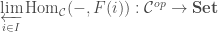
 ![\mathcal C^{op} \to \mathbf{Set}, x \mapsto \mathrm{Hom}_{[I,\mathcal C]}(\Delta(x),F)](https://s0.wp.com/latex.php?latex=%5Cmathcal+C%5E%7Bop%7D+%5Cto+%5Cmathbf%7BSet%7D%2C+x+%5Cmapsto+%5Cmathrm%7BHom%7D_%7B%5BI%2C%5Cmathcal+C%5D%7D%28%5CDelta%28x%29%2CF%29&bg=ffffff&fg=404040&s=0&c=20201002) , denoted by
, denoted by ![\mathrm{Hom}_{[I,\mathcal C]}(\Delta(-),F)](https://s0.wp.com/latex.php?latex=%5Cmathrm%7BHom%7D_%7B%5BI%2C%5Cmathcal+C%5D%7D%28%5CDelta%28-%29%2CF%29&bg=ffffff&fg=404040&s=0&c=20201002) .
.![\eta:\mathrm{Hom}_{\mathcal C}(-,L) \cong \mathrm{Hom}_{[I,\mathcal C]}(\Delta(-),F)](https://s0.wp.com/latex.php?latex=%5Ceta%3A%5Cmathrm%7BHom%7D_%7B%5Cmathcal+C%7D%28-%2CL%29+%5Ccong+%5Cmathrm%7BHom%7D_%7B%5BI%2C%5Cmathcal+C%5D%7D%28%5CDelta%28-%29%2CF%29&bg=ffffff&fg=404040&s=0&c=20201002) . Then
. Then  is a limit object of
  are the structure morphisms, i.e.
  is a terminal object in the category of cones. This is just a special case of general theorems we have proved on representable functors in virtue of the following observation:
![\mathrm{Hom}_{[I,\mathcal C]}(\Delta(-),F):\mathcal C^{op} \to \mathbf{Set}](https://s0.wp.com/latex.php?latex=%5Cmathrm%7BHom%7D_%7B%5BI%2C%5Cmathcal+C%5D%7D%28%5CDelta%28-%29%2CF%29%3A%5Cmathcal+C%5E%7Bop%7D+%5Cto+%5Cmathbf%7BSet%7D&bg=ffffff&fg=404040&s=0&c=20201002) , i.e.
, i.e. ![\mathrm{Cone}(F)=\int(\mathrm{Hom}_{[I,\mathcal C]}(\Delta(-),F))^{op}](https://s0.wp.com/latex.php?latex=%5Cmathrm%7BCone%7D%28F%29%3D%5Cint%28%5Cmathrm%7BHom%7D_%7B%5BI%2C%5Cmathcal+C%5D%7D%28%5CDelta%28-%29%2CF%29%29%5E%7Bop%7D&bg=ffffff&fg=404040&s=0&c=20201002)
![\int(\mathrm{Hom}_{[I,\mathcal C]}(\Delta(-),F))^{op}](https://s0.wp.com/latex.php?latex=%5Cint%28%5Cmathrm%7BHom%7D_%7B%5BI%2C%5Cmathcal+C%5D%7D%28%5CDelta%28-%29%2CF%29%29%5E%7Bop%7D&bg=ffffff&fg=404040&s=0&c=20201002) is an object
is an object ![\eta \in \mathrm{Hom}_{[I,\mathcal C]}(\Delta(x),F)](https://s0.wp.com/latex.php?latex=%5Ceta+%5Cin+%5Cmathrm%7BHom%7D_%7B%5BI%2C%5Cmathcal+C%5D%7D%28%5CDelta%28x%29%2CF%29&bg=ffffff&fg=404040&s=0&c=20201002) , i.e. a cone. A morphism
, i.e. a cone. A morphism  consists of a morphism
  in the category of elements
 ![\int(\mathrm{Hom}_{[I,\mathcal C]}(\Delta(-),F))](https://s0.wp.com/latex.php?latex=%5Cint%28%5Cmathrm%7BHom%7D_%7B%5BI%2C%5Cmathcal+C%5D%7D%28%5CDelta%28-%29%2CF%29%29&bg=ffffff&fg=404040&s=0&c=20201002) , i.e. a morphism
, i.e. a morphism  in
in ![\mathrm{Hom}_{[I,\mathcal C]}(\Delta(f),F))(\varepsilon)=\eta](https://s0.wp.com/latex.php?latex=%5Cmathrm%7BHom%7D_%7B%5BI%2C%5Cmathcal+C%5D%7D%28%5CDelta%28f%29%2CF%29%29%28%5Cvarepsilon%29%3D%5Ceta&bg=ffffff&fg=404040&s=0&c=20201002) , which means that
, which means that  . This is precisely the notion of a morphism of cones.
 be a functor from a small category
  exists and can be constructed as follows: Take the product
  with structure maps
  . Now for every morphism
  , so that by the universal property of the product, there is a unique morphism
  such that
  for all morphisms
  is the limit together with structure morphisms
  given by
  , where
  is the structure morphism of the equalizer.
 , showing that the
  , that is we have a cone over
  be a cone over
  . So by the universal property of the product, we get a unique morphism
  such that
  for all
  . We have for any morphism
 , we get that
  . Thus by the universal property of the equalizer
  , we get that a unique morphism
  such that
  .
. is a morphism of cones, note that
  . To see that
  be another morphism of cones, then
  satisfies
 , so that by uniqueness of
  , i.e.
  . By the uniqueness part of the universal property of the equalizer, we get that
  .
. be a functor from a small category
 is defined as follows: for an object
  ,
,  (i.e. we compose
  . This is the value of the functor
 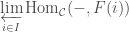 at
at ![\mathrm{Hom}_{[I, \mathcal C]}(\Delta(-),F) \cong \varprojlim_{i \in I}\mathrm{Hom}_{\mathcal C}(-,F(i))](https://s0.wp.com/latex.php?latex=%5Cmathrm%7BHom%7D_%7B%5BI%2C+%5Cmathcal+C%5D%7D%28%5CDelta%28-%29%2CF%29+%5Ccong+%5Cvarprojlim_%7Bi+%5Cin+I%7D%5Cmathrm%7BHom%7D_%7B%5Cmathcal+C%7D%28-%2CF%28i%29%29&bg=ffffff&fg=404040&s=0&c=20201002) : Both functors send an object
: Both functors send an object ![\mathrm{Hom}_{[I,\mathcal C]}(\Delta(x),F)](https://s0.wp.com/latex.php?latex=%5Cmathrm%7BHom%7D_%7B%5BI%2C%5Cmathcal+C%5D%7D%28%5CDelta%28x%29%2CF%29&bg=ffffff&fg=404040&s=0&c=20201002) is a cone with
is a cone with  , we can use the description of example C7.12:

 . Naturality is easily checked: Indeed, using the now established identifications on objects with the functor sending an object
  as an apex to the set of cones over
  to the cone with
  for each
 such that
  . The universal solution to this problem is given by the elements
 ![\mathbb{Z}[x,y]/(x^2-y^3)](https://s0.wp.com/latex.php?latex=%5Cmathbb%7BZ%7D%5Bx%2Cy%5D%2F%28x%5E2-y%5E3%29&bg=ffffff&fg=404040&s=0&c=20201002) ; this solution is universal in the sense that for every other commutative ring
; this solution is universal in the sense that for every other commutative ring ![f: \mathbb{Z}[x,y]/(x^2-y^3) \to R](https://s0.wp.com/latex.php?latex=f%3A+%5Cmathbb%7BZ%7D%5Bx%2Cy%5D%2F%28x%5E2-y%5E3%29+%5Cto+R&bg=ffffff&fg=404040&s=0&c=20201002) such that
such that  and
and  . The general definition is a straightforward abstraction from this example. Universal properties are closely related to representable functors and this relation is established by the Yoneda lemma. Understanding objects in terms of universal properties is the epitome of categorial thinking.
 be a functor.
 for some object
  . We say that
  is called a representation of
  is universal if the following property holds: For any object
  and
and  , there’s a unique morphism
  . In this case, this property is called the universal property of
  .
. are in bijection to universal elements of the form
 via
via  is an isomorphism if and only if
  is an universal element. For every object
  , but by naturality of
  ,
,  (cf. the proof of the Yoneda lemma). Thus
  is a bijection, which is just a restatement of saying that
  to the category of sets
 ![A[x]](https://s0.wp.com/latex.php?latex=A%5Bx%5D&bg=ffffff&fg=404040&s=0&c=20201002) . Concretely, we have a natural isomorphism
. Concretely, we have a natural isomorphism ![\alpha:\mathrm{Hom}_{A\textrm{-}\mathbf{CAlg}}(A[x],B) \to V(B), f \mapsto f(x)](https://s0.wp.com/latex.php?latex=%5Calpha%3A%5Cmathrm%7BHom%7D_%7BA%5Ctextrm%7B-%7D%5Cmathbf%7BCAlg%7D%7D%28A%5Bx%5D%2CB%29+%5Cto+V%28B%29%2C+f+%5Cmapsto+f%28x%29&bg=ffffff&fg=404040&s=0&c=20201002) .
. ![x \in V(A[x])](https://s0.wp.com/latex.php?latex=x+%5Cin+V%28A%5Bx%5D%29&bg=ffffff&fg=404040&s=0&c=20201002) is the corresponding universal element. This holds, because any
is the corresponding universal element. This holds, because any ![f:A[x] \to B](https://s0.wp.com/latex.php?latex=f%3AA%5Bx%5D+%5Cto+B&bg=ffffff&fg=404040&s=0&c=20201002) is given by evaluation at a uniquely determined element, namely
is given by evaluation at a uniquely determined element, namely  .
. with
with  an element
  such that the relations in
  . Consequently, for the functor
  in
in  is an universal element and
  , then consider the functor
  , i.e. from the category of left
 ![M[a]:= \{m \in M \mid am=0\}](https://s0.wp.com/latex.php?latex=M%5Ba%5D%3A%3D+%5C%7Bm+%5Cin+M+%5Cmid+am%3D0%5C%7D&bg=ffffff&fg=404040&s=0&c=20201002) . Then this functor is represented by
. Then this functor is represented by  and
and  is a universal element.
 in the arrow category is a universal element.
![[\mathcal{C},\mathbf{Set}]](https://s0.wp.com/latex.php?latex=%5B%5Cmathcal%7BC%7D%2C%5Cmathbf%7BSet%7D%5D&bg=ffffff&fg=404040&s=0&c=20201002) to
to  to
to  . Then the Yoneda lemma in this context can be stated by saying that this functor is representable by
  and the identity
  is a universal element.
 given by taking all group homomorphism to an abelian group:
  (this is a hom-functor from a larger category restricted to a subcategory). Then this functor is representable by the abelianization
 ![G^{ab}=G/[G,G]](https://s0.wp.com/latex.php?latex=G%5E%7Bab%7D%3DG%2F%5BG%2CG%5D&bg=ffffff&fg=404040&s=0&c=20201002) with the quotient map
with the quotient map  as a universal element in
  : This is the universal property of the abelianization: Every map from
  from the opposite category of topological spaces to the category of sets that sends a topological space to the set consisting of all of its open subsets. A continuous map
  . This functor is represented by the Sierpinski space
  with the topology that has as open sets
  . (For all algebraic geometers: this arises as the spectrum of a discrete valuation ring.) The open subset
  is a universal element. This reason this holds is that for any map
  , we always have
  and
and  , so the only interesting part of being continuous is requiring that
  is open. Since
  is a bijection, proving the claim.
![[\mathrm{tors}]: \mathbf{Grp} \to \mathbf{Set},G \mapsto G[\mathrm{tors}]](https://s0.wp.com/latex.php?latex=%5B%5Cmathrm%7Btors%7D%5D%3A+%5Cmathbf%7BGrp%7D+%5Cto+%5Cmathbf%7BSet%7D%2CG+%5Cmapsto+G%5B%5Cmathrm%7Btors%7D%5D&bg=ffffff&fg=404040&s=0&c=20201002) . (This defines a functor because group homomorphisms send torsion elements to torsion elements.) Suppose that
. (This defines a functor because group homomorphisms send torsion elements to torsion elements.) Suppose that ![[\mathrm{tors}]](https://s0.wp.com/latex.php?latex=%5B%5Cmathrm%7Btors%7D%5D&bg=ffffff&fg=404040&s=0&c=20201002) is represented by a group
is represented by a group ![g \in G[\mathrm{tors}]](https://s0.wp.com/latex.php?latex=g+%5Cin+G%5B%5Cmathrm%7Btors%7D%5D&bg=ffffff&fg=404040&s=0&c=20201002) be a universal element. Then for every
be a universal element. Then for every  , we have an element
 ![\overline{1} \in \mathbb{Z}/n\mathbb{Z}[\mathrm{tors}]](https://s0.wp.com/latex.php?latex=%5Coverline%7B1%7D+%5Cin+%5Cmathbb%7BZ%7D%2Fn%5Cmathbb%7BZ%7D%5B%5Cmathrm%7Btors%7D%5D&bg=ffffff&fg=404040&s=0&c=20201002) . By universality of
. By universality of  that sends
  . But this implies that
  .
.
 . Then both
  are morphisms
  , so they must agree, thus
  . By symmetry,
  proving that
  consisting of an element
  .
. are morphisms
  .
. both satisfy the universal property for a functor
  .
. . For two such functors, we can consider natural transformations between them, which we can compose in an associative way. For any functor, there’s the identity natural transformation. So this turns the collection of functors
 ![[\mathcal C,\mathcal D]](https://s0.wp.com/latex.php?latex=%5B%5Cmathcal+C%2C%5Cmathcal+D%5D&bg=ffffff&fg=404040&s=0&c=20201002) has as its objects all functors
has as its objects all functors  and as morphisms natural transformations, with composition of natural transformations defined pointwise.
![[G,\mathbf{Set}]](https://s0.wp.com/latex.php?latex=%5BG%2C%5Cmathbf%7BSet%7D%5D&bg=ffffff&fg=404040&s=0&c=20201002) for a group
for a group ![[G,k\mathrm{-Vect}]](https://s0.wp.com/latex.php?latex=%5BG%2Ck%5Cmathrm%7B-Vect%7D%5D&bg=ffffff&fg=404040&s=0&c=20201002) is the category of representations of
is the category of representations of  be a functor, then the map
 ![\varphi^{x,F}:\mathrm{Hom}_{[\mathcal C,\mathbf{Set}]}(\mathrm{Hom}_{\mathcal C}(x,-),F) \to F(x), \eta \mapsto \eta_{x}(\mathrm{id}_x)](https://s0.wp.com/latex.php?latex=%5Cvarphi%5E%7Bx%2CF%7D%3A%5Cmathrm%7BHom%7D_%7B%5B%5Cmathcal+C%2C%5Cmathbf%7BSet%7D%5D%7D%28%5Cmathrm%7BHom%7D_%7B%5Cmathcal+C%7D%28x%2C-%29%2CF%29+%5Cto+F%28x%29%2C+%5Ceta+%5Cmapsto+%5Ceta_%7Bx%7D%28%5Cmathrm%7Bid%7D_x%29&bg=ffffff&fg=404040&s=0&c=20201002) is a bijection that is natural in
is a bijection that is natural in  as follows: let
  , then set
  to be the following natural transformation: for any object
  and any morphism
  , we need to check that this is indeed a natural transformation from
  to
to  be a third object and let
  be a morphism in
 , then
  showing that the diagram commutes. Hence
  is a natural transformation.
 . Let
. Let  be a natural transformation, then we need to show that
  , which we can check this component-wise. Let
  by naturality of
  , see the diagram below, applied to the identity on
 . This shows that
  and
and  are mutually inverse bijections. Naturality in
  be a functor, i.e. a contravariant functor on
 ![\mathrm{Hom}_{[\mathcal{C}^{op},\mathbf{Set}]}(\mathrm{Hom}_{\mathcal C}(-,x),F) \to F(x), \eta \mapsto \eta_x(\mathrm{id}_x)](https://s0.wp.com/latex.php?latex=%5Cmathrm%7BHom%7D_%7B%5B%5Cmathcal%7BC%7D%5E%7Bop%7D%2C%5Cmathbf%7BSet%7D%5D%7D%28%5Cmathrm%7BHom%7D_%7B%5Cmathcal+C%7D%28-%2Cx%29%2CF%29+%5Cto+F%28x%29%2C+%5Ceta+%5Cmapsto+%5Ceta_x%28%5Cmathrm%7Bid%7D_x%29&bg=ffffff&fg=404040&s=0&c=20201002) is a natural bijection.
is a natural bijection. be objects. Then there is a natural isomorphism
 ![\mathrm{Hom}_{[\mathcal{C}^{op},\mathbf{Set}]}(\mathrm{Hom}_{\mathcal C}(-,x),\mathrm{Hom}_{\mathcal C}(-,y)) \cong \mathrm{Hom}_{\mathcal C}(x,y)](https://s0.wp.com/latex.php?latex=%5Cmathrm%7BHom%7D_%7B%5B%5Cmathcal%7BC%7D%5E%7Bop%7D%2C%5Cmathbf%7BSet%7D%5D%7D%28%5Cmathrm%7BHom%7D_%7B%5Cmathcal+C%7D%28-%2Cx%29%2C%5Cmathrm%7BHom%7D_%7B%5Cmathcal+C%7D%28-%2Cy%29%29+%5Ccong+%5Cmathrm%7BHom%7D_%7B%5Cmathcal+C%7D%28x%2Cy%29&bg=ffffff&fg=404040&s=0&c=20201002) given by
given by  .
.![Y_{\mathcal C}: \mathcal C \to [\mathcal C^{op},\mathbf{Set}]](https://s0.wp.com/latex.php?latex=Y_%7B%5Cmathcal+C%7D%3A+%5Cmathcal+C+%5Cto+%5B%5Cmathcal+C%5E%7Bop%7D%2C%5Cmathbf%7BSet%7D%5D&bg=ffffff&fg=404040&s=0&c=20201002) , called the Yoneda embedding, given by
, called the Yoneda embedding, given by  is fully faithful.
 and
and  are naturally isomorphic, then
  are naturally isomorphic, then
 ![[\mathcal C^{op},\mathbf{Set}]](https://s0.wp.com/latex.php?latex=%5B%5Cmathcal+C%5E%7Bop%7D%2C%5Cmathbf%7BSet%7D%5D&bg=ffffff&fg=404040&s=0&c=20201002) , containg as objects all Hom-functors and as morphisms natural transformations between them.
, containg as objects all Hom-functors and as morphisms natural transformations between them. , given by pulling back along the projection
  . In this sense, the projection
  is the universal morphism that restricts to
  , the localization
  together with the canonical morphism
  is the universal solution to the problem of finding a ring
  such that
  .
.
 by the Yoneda lemma. This is a conceptually very satisfying proof, as we didn’t have to fiddle with equivalence classes or fractions, but we only used the abstract defining properties of localizations and quotients.
 , then
  .
. is the multiplicatively closed subset generated by
  using the Yoneda lemma.
 , between two categories
  , one has a morphism
  . In this situation, the notion of a natural transformation conceptualizes what it means for this collection of morphisms to vary “naturally” with the object
  consists of the following data:
 called the component of
  which means that
 . Then a natural transformation
  has only one component, as
  (i.e. for any morphism in
  , (by abuse of notation, we write
  correspond to morphisms of representations.
 be the category of monoids. Fix
  . Let
. Let  be the functor that sends a commutative ring to the multiplicative monoid of the matrix ring:
  . Every ring homomorphism
  induces a monoid homomorphism
  of multiplicative monoids by applying
  be the “forgetful” functor that forgets about addition and sends a commutative ring to its multiplicative monoid. Every ring homomorphism respects multiplication and the unit element, so that it induces a monoid homomorphism on the multiplicative monoids. The determinant is defined by a polynomial with coefficients in
  . Hence it doesn’t matter if we apply the ring homomorphism
  stating that the determinant is natural in
![H:[0,1] \times X \to Y](https://s0.wp.com/latex.php?latex=H%3A%5B0%2C1%5D+%5Ctimes+X+%5Cto+Y&bg=ffffff&fg=404040&s=0&c=20201002) such that
such that  for all
  for all
  .
.![[0,1]](https://s0.wp.com/latex.php?latex=%5B0%2C1%5D&bg=ffffff&fg=404040&s=0&c=20201002) as a time parameter, as in the picture above. The definition states that
as a time parameter, as in the picture above. The definition states that  like
like  like
like  and three morphisms: the two identities and a unique morphism
  consists of the following data:
 and
and  , we have
 be functors. Then a “categorical homotopy” from
  such that
  for all
  for all
  in
in  and
and  . This means that on the subcategory
  ,
,  ,
,  be functors, then natural transformations
  as follows:
 and
and  .
. and let
  and let
  (the last equality holds by naturality of

 is indeed a functor. It is clear from the construction that
  is a categorical homotopy from
  for all
  . Naturality now follows from functoriality of
 such that
  and
and  are the identity functors on
  such that
  are homotopic to the identities on
  .
. and
and  , the induced map
  is injective.
 and
and  are isomorphic in
  with inverse
  , then there are some
  such that
  and
and  as the induced maps on
  -sets is surjective. We get
  , so
, so  , so
, so  be functors and let
  is a bijection with inverse given by
  .
. , which implies that
  From this equation, we conclude that the maps induced by
  , hence one is injective, surjective or bijective if and only if the other one is.
 are functors such that
  , there is an object
  such that
  such that
  , showing that
  such that
  is isomorphic to
  . Let
. Let  is a morphism
  . By full faithfulness of
  such that
  .
. , such that by faithfulness of
  . As for identities, we get for any object
  so that by faithfulness,
  .
. so that
  .
. is naturally isomorphic to
  such that for any morphism
  . Now as
  such that
  . To show that
  is natural, insert into
  which implies by functionariality
  so that by faithfulness, we get
  , which means precisely that
  is an isomorphism for each
  is an isomorphism. (If
 a map
a map 
 we have
 and morphisms
  we have
  .
. has to send the unique object of
  determines a functor if and only if it preserves the monoid operation and the identity, i.e. if and only if it is a monoid homomorphisms. Thus for monoids (and hence for groups), we can regard homomorphisms as functors.
 . Since
  such that
  and
and  . These are precisely the axioms for a group action on
  is a field and we consider the category
  of vector spaces over
  correspond to representations of
  be the category of pointed smooth manifolds, i.e. objects are pairs
  where
where  and morphisms
  are smooth maps
  . Then there’s the tangent space functor
  to the category of
  of
of  to the differential
  . The fact that this behaves functorially is an abstract version of the chain rule:
  , justifying the assertion on functoriality in calculus above.
 be the category of rings with ring homomorphisms as morphisms, then for any ring
  form a group and ring homomorphisms preserve units so that a ring homomorphism
  . We obtain a functor from
  . The fact that this is a functor is even part of the Eilenberg-Steenrod axioms for homology theories.
 that equips a topological space with its Borel
  -algebra, turning it into a measurable space. Every continuous map is measurable with respect to the corresponding Borel
  which is an abelian group. One could hope that this can be made into a functor. The problem is that central elements don’t necessarily get sent to central elements under a group homomorphism. Indeed, it is impossible to define any action on morphisms such that the assignment on objects
  becomes a functor, for the identity on the cyclic group on two elements
  factors through the inclusion
  as a transposition and the sign homomorphism
  . We have
  . However, the center of
  implying that the identity on
  , we have a set
  and for a morphism
  , we can postcompose with
  . By associativity of composition and the definition of the identity elements, this construction yields a functor
 , we set
  composition is defined like the composition in
  .
. can be made into a functor in two different ways, a covariant one and a contravariant one. For the covariant one, let
  via
via  , giving rise to the covariant powerset functor. For the contravariant one, we can define for a map
  via
via  . In both cases the verification of the functorial properties is easy.
 , set
, set  and for a (necessarily injective) morphism
  , define
  . The transitivity formula for norms in towers translates into functoriality of this construction: For a tower of extensions
  we have
  .
. form a C*-algebra with pointwise operations (i.e. addition, multiplication, scalar multiplication and conjugation), denoted by
  . If
. If  ,
,  . We obtain a contravariant functor from the category of compact Hausdorff spaces to the category of commutative unital C*-algebras.
 and for a morphism
  , we get a map
  . This construction is a functor, called the contravariant Hom functor.
 , a set of morphisms
 , a map
  called composition and denoted by
 , there exists an identity
  such that for all objects
  and all morphisms
  we have
  and
and 
 and
and  , we have
 unless
  and
and 
 is the class of all sets and for
  ,
,  is the set of all maps from
  is the category consisting of all sets as objects, and for two objects
  ,
,  is the set of all relations from
  . Given three sets
  , we can form the composite relation
  . (If
. (If  and the only morphisms are the identity morphisms required by the definition of categories. Due to the striking similarity with discrete topological spaces (compare for instance the set of morphisms
  if
if  and
and  if
if  with the discrete metric), this construction is called the discrete category on the set
  . But the requirements for compositions and identities force a relation to have some properties if it is supposed to define a category in this manner: the existence of identity morphisms in the supposed category is equivalent to the relation being reflexive and the existence of compositions translates to transivity. A reflexive and transitive relation is called “preorder”. For instance, all equivalence relations and all partial orderings are preorders. An example of a preorder that is neither can be formed by taking a ring, say, an integral domain
  and
and  . If there is such a morphism, then
  and
and  . Then composition is a (totally defined) mapping
  , i.e. a binary operation.
 implies that
  is a unit with respect to this binary operation and the associativity of the composition implies that the binary operation is, well, associative. Thus composition
  makes
makes  and defining the composition via the monoid operation. These constructions are inverse to each other, such that monoids correspond to one-object categories.
 be the category having elements from
  , such that
  is in bijection with
  . This groupoid played an important role in a
  has as its objects all elements of
  ,
,  consists of all homotopy classes of paths from
 ![k[G]](https://s0.wp.com/latex.php?latex=k%5BG%5D&bg=ffffff&fg=404040&s=0&c=20201002) -module, then the dual space
-module, then the dual space  is a
is a  . This is called the dual representation.
 , where we regard
  is an anti-isomorphism, i.e. an isomorphism
  , as
, as  , which means that inversion
  , now if we compose the functors
  , we get a covariant functor
  is a
is a  .
. induces a ring homomorphism
 ![k[G] \to k[G\times G]\cong k[G] \otimes_k k[G]](https://s0.wp.com/latex.php?latex=k%5BG%5D+%5Cto+k%5BG%5Ctimes+G%5D%5Ccong+k%5BG%5D+%5Cotimes_k+k%5BG%5D&bg=ffffff&fg=404040&s=0&c=20201002) given on basis elements by
given on basis elements by  (this is called “comultiplication” in the setting of Hopf algebras) and that
 ![k[G] \otimes_k k[G]](https://s0.wp.com/latex.php?latex=k%5BG%5D+%5Cotimes_k+k%5BG%5D&bg=ffffff&fg=404040&s=0&c=20201002) -module (where the first copy of
-module (where the first copy of ![k[G] \to k[G] \otimes_k k[G]](https://s0.wp.com/latex.php?latex=k%5BG%5D+%5Cto+k%5BG%5D+%5Cotimes_k+k%5BG%5D&bg=ffffff&fg=404040&s=0&c=20201002) .
. is a
is a  is defined via
![\mathrm{Hom}_k(V,W)^G=\mathrm{Hom}_{k[G]}(V,W)](https://s0.wp.com/latex.php?latex=%5Cmathrm%7BHom%7D_k%28V%2CW%29%5EG%3D%5Cmathrm%7BHom%7D_%7Bk%5BG%5D%7D%28V%2CW%29&bg=ffffff&fg=404040&s=0&c=20201002) .
. given on elementary tensors by
  is an isomorphism of
 ![\mathrm{dim}_k\mathrm{Hom}_{k[G]}(V,W)/ \mathrm{dim}_k \mathrm{End}_{k[G]}(V)](https://s0.wp.com/latex.php?latex=%5Cmathrm%7Bdim%7D_k%5Cmathrm%7BHom%7D_%7Bk%5BG%5D%7D%28V%2CW%29%2F+%5Cmathrm%7Bdim%7D_k+%5Cmathrm%7BEnd%7D_%7Bk%5BG%5D%7D%28V%29&bg=ffffff&fg=404040&s=0&c=20201002) (cf. 3.19)
(cf. 3.19) ,
,  is a linear projection.
 is well-defined note that for
  , we get
  , since the map
  is a bijection. That
  and linearity is clear.
 and
and  be finite-dimensional, then
 ![\mathrm{dim}_k \mathrm{Hom}_{k[G]}(V,W)=\frac{1}{|G|}\sum_{g \in G}\mathrm{Tr}(\rho_V(g^{-1})) \mathrm{Tr}(\rho_W(g))](https://s0.wp.com/latex.php?latex=%5Cmathrm%7Bdim%7D_k+%5Cmathrm%7BHom%7D_%7Bk%5BG%5D%7D%28V%2CW%29%3D%5Cfrac%7B1%7D%7B%7CG%7C%7D%5Csum_%7Bg+%5Cin+G%7D%5Cmathrm%7BTr%7D%28%5Crho_V%28g%5E%7B-1%7D%29%29%C2%A0%5Cmathrm%7BTr%7D%28%5Crho_W%28g%29%29&bg=ffffff&fg=404040&s=0&c=20201002)
![\mathrm{avg}:\mathrm{Hom}_k(V,W) \to \mathrm{Hom}_k(V,W)^G = \mathrm{Hom}_{k[G]}(V,W)](https://s0.wp.com/latex.php?latex=%5Cmathrm%7Bavg%7D%3A%5Cmathrm%7BHom%7D_k%28V%2CW%29+%5Cto+%5Cmathrm%7BHom%7D_k%28V%2CW%29%5EG+%3D+%5Cmathrm%7BHom%7D_%7Bk%5BG%5D%7D%28V%2CW%29&bg=ffffff&fg=404040&s=0&c=20201002) ,
,  is a projection onto the subspace
  (by 5.6), we get that
 ![\mathrm{dim}_k \mathrm{Hom}_{k[G]}(V,W) = \mathrm{Tr}(\mathrm{avg})](https://s0.wp.com/latex.php?latex=%5Cmathrm%7Bdim%7D_k+%5Cmathrm%7BHom%7D_%7Bk%5BG%5D%7D%28V%2CW%29+%3D+%5Cmathrm%7BTr%7D%28%5Cmathrm%7Bavg%7D%29&bg=ffffff&fg=404040&s=0&c=20201002) . Using the isomorphism
. Using the isomorphism  (by 5.5), we get that
  . Using properties of traces and the definition of the dual representation, this equals
  .
.![\mathrm{dim}_k \mathrm{Hom}_{k[G]}(V,W)](https://s0.wp.com/latex.php?latex=%5Cmathrm%7Bdim%7D_k%C2%A0%5Cmathrm%7BHom%7D_%7Bk%5BG%5D%7D%28V%2CW%29&bg=ffffff&fg=404040&s=0&c=20201002) and
and ![\mathrm{dim}_k \mathrm{End}_{k[G]}(V)](https://s0.wp.com/latex.php?latex=%5Cmathrm%7Bdim%7D_k+%5Cmathrm%7BEnd%7D_%7Bk%5BG%5D%7D%28V%29&bg=ffffff&fg=404040&s=0&c=20201002) (cf. the discussion preceeding 5.6). But now 5.7 gives us an expression for these dimension that only involves the traces
(cf. the discussion preceeding 5.6). But now 5.7 gives us an expression for these dimension that only involves the traces  and
and  . It thus makes sense to give a special name to the function
 is called the character of
  . (Note that the trace of a matrix is invariant under conjugation, so the character doesn’t depend on a choice of basis for